Прогнозирование пород собак с Керасом

- Использование подхода к трансферному обучению (VGG16 И InceptionV3)

Где находится набор данных? Из Kaggle~

Данные состоят из 10222 изображений собак 120 различных пород, каждый каталог содержит изображения только одной породы собак.

Прежде всего, давайте изучим наши данные

import numpy as np
import pandas as pd
import seaborn as sns
import sklearn as sklearn
import matplotlib.pyplot as plt
%matplotlib inline
# loading the CSV File with pandas
labels = pd.read_csv('labels.csv')
submission = pd.read_csv('sample_submission.csv')
# checking is there any missing value
labels.isnull().values.any()
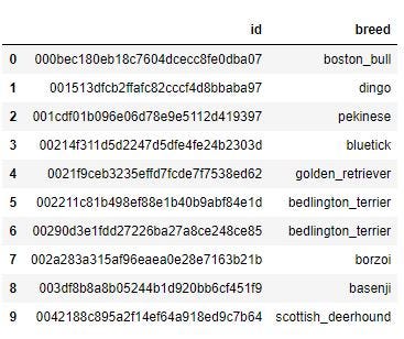
# check first 10 rows of data
labels.head(10)

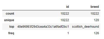
# take a look the basic information 
labels.describe(include="all")

Во-вторых, давайте сделаем визуализацию данных для лучшего понимания данных.

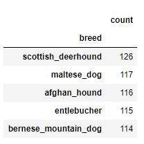
Сводная таблица — отображение каждой породы в порядке убывания

breed_counts = pd.pivot_table(labels, index=['breed'], aggfunc='count')
# rename the column
breed_counts = breed_counts.rename(columns = {"id" : "count"})
# show in desending order 
breed_counts = breed_counts.sort_values("count", ascending=False)
# show top 5 rows
breed_counts.head()

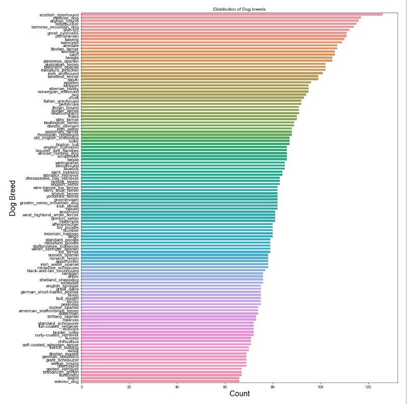
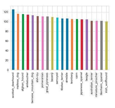
Визуализация распределения обучающих данных

fig, ax = plt.subplots()
fig.set_size_inches(15,18)
sns.set_style("whitegrid")
ax = sns.barplot(x = breed_counts['count'], y = breed_counts.index, data = labels)
ax.set_yticklabels(ax.get_yticklabels(), fontsize = 12)
ax.xaxis.label.set_size(20)
ax.yaxis.label.set_size(20)
ax.set(xlabel='Count',ylabel='Dog Breed')
ax.set_title('Distribution of Dog breeds')

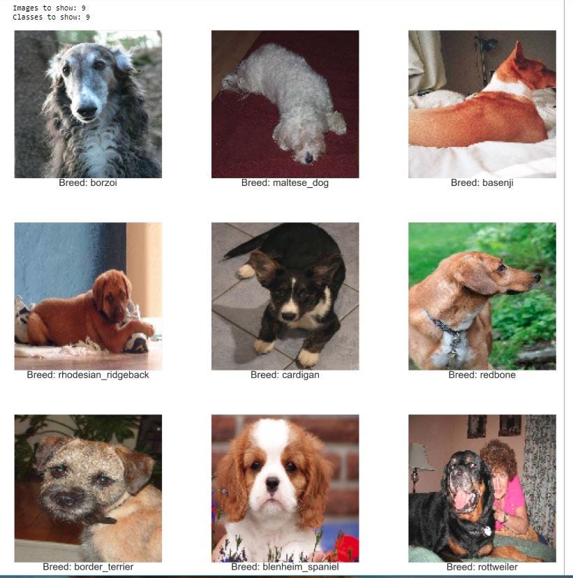
В-третьих, загрузка соответствующих изображений

from tqdm import tqdm
import cv2
# Helper-function for plotting images
def plot_images(images, classes):
    assert len(images) == len(classes) == 9
    
    # Create figure with 3x3 sub-plots.
    fig, axes = plt.subplots(3, 3,figsize=(60,60),sharex=True)
    fig.subplots_adjust(hspace=0.3, wspace=0.3)
   
    for i, ax in enumerate(axes.flat):
        # Plot image.
        
        ax.imshow(cv2.cvtColor(images[i], cv2.COLOR_BGR2RGB).reshape(img_width,img_height,3), cmap='hsv')    
        xlabel = "Breed: {0}".format(classes[i])
    
        # Show the classes as the label on the x-axis.
        ax.set_xlabel(xlabel)
        ax.xaxis.label.set_size(60)
        # Remove ticks from the plot.
        ax.set_xticks([])
        ax.set_yticks([])
    
    # Ensure the plot is shown correctly with multiple plots
    # in a single Notebook cell.
    
    plt.show()

Прочитайте все изображения в обучающем наборе данных, используя цикл for для значений файлов csv:

# I have also set an im_width variable which sets the size for the image to be re-sized to, 128x128 px
img_width = 128
img_height = 128
images = []
classes = []
# load training images
for f, breed in tqdm(labels.values):
    img = cv2.imread('C:/Users/shell/Desktop/Project-1/train/{}.jpg'.format(f))
    classes.append(breed)
    images.append(cv2.resize(img, (img_width, img_height)))
# plot some example images
# select random images
from random import randint
random_numbers = [randint(0, len(images)) for p in range(0,9)]
images_to_show = [images[i] for i in random_numbers]
classes_to_show = [classes[i] for i in random_numbers]
print("Images to show: {0}".format(len(images_to_show)))
print("Classes to show: {0}".format(len(classes_to_show)))
# plot the images
plot_images(images_to_show, classes_to_show)

Наконец, сократите количество пород со 120 до 20 для моделей

from sklearn.model_selection import train_test_split
# reduce size to 20
num_breeds = 20
top_breeds = sorted(list(labels['breed'].value_counts().head(num_breeds).index))
sub_train_top_breeds = labels[labels['breed'].isin(top_breeds)]
# plot
sub_train_top_breeds.breed.value_counts().plot(kind='bar')
print(top_breeds)

Сопоставление пород собак:

# I will put the 20 breeds in a key-value pair
map_characters = {0:'afghan_hound', 1:'airedale', 2:'australian_terrier', 3:'basenji', 4:'beagle', 5:'bernese_mountain_dog', 
                  6:'blenheim_spaniel', 7:'cairn', 8:'entlebucher', 9:'great_pyrenees', 10:'irish_wolfhound', 11:'japanese_spaniel', 
                  12:'leonberg',13:'maltese_dog', 14:'miniature_pinscher', 15:'pomeranian', 16:'samoyed', 17:'scottish_deerhound', 
                  18:'shih-tzu', 19:'tibetan_terrier'}

Маркировка данных — одно горячее кодирование

# we do one hot encoding to lableing the data
targets_series = pd.Series(sub_train_top_breeds['breed'])
one_hot = pd.get_dummies(targets_series, sparse = True)
one_hot_labels = np.asarray(one_hot)
print(one_hot_labels)
# I have also set an im_size variable which sets the size for the image to be re-sized to, 128*128 px
im_size = 164
x_train = []
y_train = []
# loading the training data of all the images in the 20 breeds, using a for loop through the values of the csv files.
i = 0
for f, breed in tqdm(sub_train_top_breeds.values):
    img = cv2.imread('C:/Users/shell/Desktop/Project-1/train/{}.jpg'.format(f))
    label = one_hot_labels[i]
    x_train.append(cv2.resize(img, (im_size, im_size)))
    y_train.append(label)
    i += 1
# we do the normolize for the image data in order to make it easier for nerual networks to learn 
x_train_raw = np.array(x_train, np.float32) / 255.
y_train_raw = np.array(y_train, np.uint8)
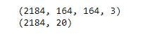
# check the shape of the ouputs to make sure everything went as expected
print(x_train_raw.shape)
print(y_train_raw.shape)

Разделить на тестирование и обучение

# split data into test and train
x_train,x_test,y_train,y_test = train_test_split(x_train_raw, y_train_raw, test_size=0.3, random_state=1)

Построить модель (перенос обучения)

Что такое трансферное обучение?

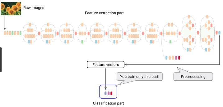
Трансферное обучение включает в себя подход, при котором знания, полученные в одной или нескольких исходных задачах, передаются и используются для улучшения изучения связанной целевой задачи, в простом предложении — является повторным использованием предварительно обученной модели для новой задачи. .

При трансферном обучении мы в основном пытаемся использовать то, что было изучено в одной задаче, для улучшения обобщения в другой. Мы переносим веса, полученные сетью в Задаче А, в новую Задачу Б.

Как это работает?

Мы пытаемся перенести как можно больше знаний из предыдущей задачи, на которой обучалась модель, в новую задачу.

Почему мы его используем?

Самым большим преимуществом является экономия времени на обучение, поскольку в большинстве случаев нейронная сеть работает лучше, и вам не нужно много данных, что становится еще одним преимуществом — меньше данных.

Именно здесь в игру вступает трансферное обучение, потому что с его помощью вы можете построить надежную модель машинного обучения со сравнительно небольшим объемом обучающих данных, поскольку модель уже предварительно обучена.

1. VGG16

Нейронная сеть VGG — это классификация изображений, сверточная нейронная сеть. Учитывая изображение, сеть VGG выводит вероятности различных классов, которым потенциально может принадлежать изображение.

Загрузить библиотеки

from keras.applications.vgg16 import VGG16
from keras import optimizers
from keras.models import Model
from sklearn import preprocessing

Создайте предварительно обученную модель

# Create the pre-trained model
base_model = VGG16(weights='imagenet', include_top=False, input_shape=(im_size, im_size, 3))

Добавить верхние слои

x = base_model.output
x = Flatten()(x)
predictions = Dense(num_class, activation='softmax')(x)

Модель, которую мы будем обучать

model = Model(inputs = base_model.input, outputs=predictions)
# First: train only the top layers (which were randomly initialized)
for layer in base_model.layers:
    layer.trainable = False
# compile model
model.compile(loss='categorical_crossentropy', 
              optimizer='adam', 
              metrics=['accuracy'])
callbacks_list = [keras.callbacks.EarlyStopping(monitor='val_acc', patience = 3, verbose = 1)]
model.summary()

Подобрать модель

# fit in the model and use epochs = 5
model.fit(x_train,y_train, epochs = 5, validation_data = (x_test,y_test), 
          verbose = 1,callbacks = [MetricsCheckpoint('logs')])
score = model.evaluate(x_test, y_test, verbose = 0)
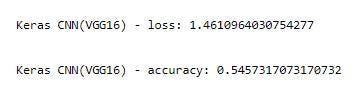
print('\nKeras CNN(VGG16) - loss:', score[0], '\n')
print('\nKeras CNN(VGG16) - accuracy:', score[1], '\n')

prediction = model.predict(x_test)
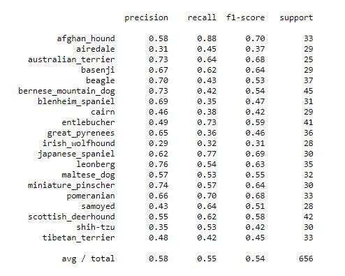
print('\n', sklearn.metrics.classification_report(np.where(y_test > 0)[1], np.argmax(prediction, axis = 1), target_names=list(map_characters.values())), sep='')

Визуализируйте кривую обучения и матрицу путаницы

y_pred_classes = np.argmax(prediction,axis = 1) 
y_true = np.argmax(y_test,axis = 1) 
confusion_mtx = confusion_matrix(y_true, y_pred_classes)
plotKerasLearningCurve()
plt.show()
plot_confusion_matrix(confusion_mtx, classes = list(map_characters.values()))
plt.show()

Вывод. Мы получили точность 54,57 % на основе 20 топовых пород, но должны еще улучшить производительность, возможно, используя больше эпох и проанализировав все 120 пород, это улучшит результаты.

Начальная версия 3

Сеть Inception стала важной вехой в развитии классификаторов CNN. Вы можете использовать эту модель, переобучив последний слой в соответствии с вашими требованиями к классификации.

from keras.applications import inception_v3
from keras.applications.inception_v3 import InceptionV3
from keras.applications.inception_v3 import preprocess_input as inception_v3_preprocessor
from keras.layers import Dense, GlobalAveragePooling2D

Получить базовую модель

# Get the InceptionV3 model so we can do transfer learning
im_width = 164
im_height = 164
base_model = InceptionV3(weights = 'imagenet', pooling='avg', include_top = False, input_shape = (im_width, im_height, 3))

Добавить слой объединения глобальных пространственных средних

x = base_model.output
x = GlobalAveragePooling2D()(x)
# Add a fully-connected layer and a logistic layer with 20 classes

Добавить полносвязный слой и логистический уровень с 20 классами

x = Dense(512, activation='relu')(x)
x = Dropout(0.5)(x)
predictions = Dense(num_class, activation = 'softmax')(x)

Построить модель обучения

# This is the model we will train
model = Model(inputs = base_model.input, outputs = predictions)

Обучать только верхние слои

# first: train only the top layers i.e. freeze all convolutional InceptionV3 layers
for layer in base_model.layers:
    layer.trainable = False

Скомпилировать с «Адамом»

# Compile with Adam
model.compile(loss='categorical_crossentropy', 
              optimizer='adam',
              metrics=['accuracy'])

Обучить модель

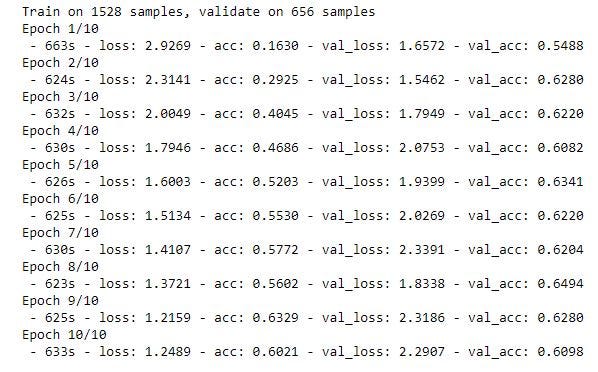
model.fit(x_train, y_train,  epochs = 10, validation_data = (x_test,y_test), verbose = 2, callbacks = [MetricsCheckpoint('logs')])

Оцените модель

score = model.evaluate(x_test, y_test, verbose = 0)
print('\nKeras CNN(InceptionV3) - loss:', score[0], '\n')
print('\nKeras CNN(InceptionV3) - accuracy:', score[1], '\n')

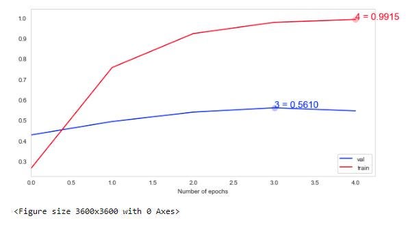
Визуализируйте кривую обучения и матрицу путаницы

y_pred_classes = np.argmax(prediction,axis = 1) 
y_true = np.argmax(y_test, axis = 1)
confusion_mtx = confusion_matrix(y_true, y_pred_classes)
plotKerasLearningCurve()
plt.show()
plot_confusion_matrix(confusion_mtx, classes = list(map_characters.values()))
plt.show()

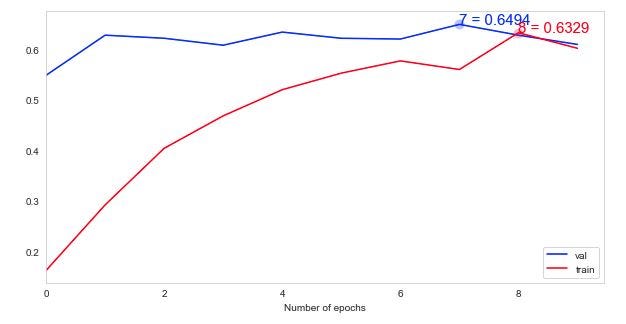
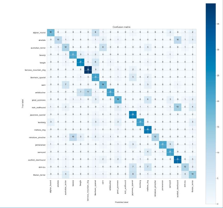
Вывод. Мы получили точность 60,98 % на основе 20 топовых пород, но должны еще улучшить производительность, возможно, используя больше эпох. и запустить все 120 пород должны улучшить результаты.

Сравните модель VVG16 VS InceptionV3

InceptionV3 имеет немного лучший показатель точности, который составляет 60,98% на основе 20 лучших пород собак.